The past couple of weeks have seen small but significant steps on the development towards the retooling my sim model for AFL.
The first thing I had to do was update my historical data from, the AFL Tables scrapings.
For that I dragged out my old parsing code which still works, but had to deal with the fact that I had stored the goals/behinds with a dot separator. Which is actually not really a good idea if you’re generating a CSV (comma separated value) file, as if you load those straight into Excel the trailing zero may get stripped, so 10 behinds would be come 1 behind.
It’s OK for my purposes since I do most of my stuff in Python, but I decided that I would make my history file public I should at least eliminate that misunderstanding, and so for those fields I’ve changed the sub-separator to the underscore ( _ ).
After all that cleaning up it’s at a point where I can make the history file public, so you can now pick it up on the new Resources section, which may get expanded with other files that I decide to make public.
With that dataset sorted out, I could get stuck into analysing that.
In previous years I’d used the normal distribution (ye olde bell curve) as the basis for the simulation module. There are a few of problems with that, the most annoying to me is that it would generate negative scores.
Anyway, while I was attempting to work up a plausible sim model for “sokkah”, in that case I reasoned that the poisson distribution was most appropriate there as it was an event-based sport, after all.
AFL scoring, too, is a series of events, but with goals and behinds, the waters get muddied a bit as far as the quantum of the data. I guess I still couldn’t get away from the idea of using a continuous distribution, but for that I decided to use the continuous equivalent of the poisson distribution, the gamma curve.
So, I applied that to the set of final scores in the AFL/VFL set, and it worked marvelously.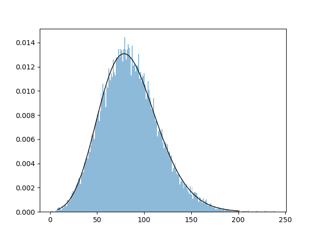
So that’s what we’ll be using as a basis. I’ve also gotten the suggestion that the log-normal curve might also be worthy as it exhibits similar characteristics, so that might get a look in as I fine-tune things.
I’m now at the point where I’m trying to calibrate forecast results (based on the GRAFT system) against actual results, and that’s actually not looking so great. As far as margins go, what I’ve found is that while there is a good correlation in one sense (bigger predicted margins match up with bigger actual margins), the average of the actual margins for each slice is about 75-76% of the forecast margin. Not that flash. I can generate a pretty good win probability system out of it, but I also want to nail the “line” margins and par scores as well.
In other words, for games where I have “predicted” one team to win by 50 points, they end up winning (on average) by 38 (mean) or 40 (median) points – albeit with a lot of outliers as you’d expect.
There’s a bit of thinking here to do, and I strongly suspect that it’ll lead to a significantly reworking of the GRAFT system to the point where it’ll have to be considered Version 3 – but what that actually entails is still a bit of a mystery. It may be that this will be a whole new system that moves away from the linear arithmetic model, at least in part.
So that’s where we’re up to at this point. How much of this work I can get done before the new season is a little uncertain, because there’s a few other things on my plate over the next few months. But we’ll see how we go.